実践手話認識 - モデル開発編 補足: 時系列認識における Loss 計算のハマりどころ

Thumbnail image
This image is generated with ChatGPT-4 Omni, and edited by the author.
作成日: 2024年09月12日(木) 00:00
最終更新日: 2024年09月18日(水) 09:47
カテゴリ: 手話言語処理
タグ:  実践手話認識 深層学習 時系列認識

Encoder-Decoder を用いて Loss 計算を行う際のハマりどころについて説明します.

こんにちは.高山です.
今回の記事は,Encoder-Decoder を用いた時系列認識の処理 (以降では Encoder-Decoder 解説記事と記載します) の補足になります.

Encoder-Decoder 解説記事では,基本的な構成や動作,および学習ループなどの全体的な構成に注力して説明しました.
Loss 計算などの細かな点については,あまり触れなかったので本記事で補足説明をさせていただきたいと思います.

時系列認識の Loss 計算はいくつかのハマりどころがあります.
今回の記事では,下記の 3 点について説明したいと思います.

  • Loss 計算時のインデクス調整
  • Nan に対する対処
  • ラベル系列長を用いた Loss の正規化

簡単な検証コードや学習に使えるクラスも紹介しますので,実際に動かして確認してみると理解しやすいと思います.

更新履歴 (大きな変更のみ記載しています)

  • 2024/09/18: カテゴリを変更しました
  • 2024/09/17
    • タイトルとタグサマリを更新しました
    • 系列認識 (Sequential recognition) は別の手法を連想させる可能性があるので,時系列認識 (temporal recognition) という用語を用いるようにしました

1. Loss計算時のインデクス調整

Encoder-Decoderの解説記事で,時系列認識では Decoder に 1 個のラベルを入力して,次のラベルを予測させると述べました.
図1に学習時における Decoder の動作を示します.

図1: Lossのインデクス調整
Lossのインデクス調整

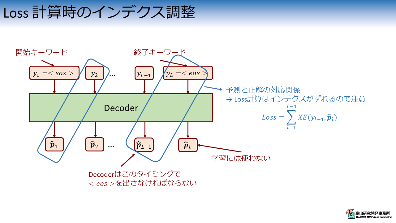
Decoder に正解ラベル系列から取り出した 1 個のラベル \(y_l\) を入力した場合を考えます.
このときの Decoder の出力 \(\hat{\boldsymbol{p}_{l}}\) は次のラベルの予測確率を示しています.
(正確には確率化する前の応答値ですが,分かりにくいと思いますので確率という単語を用います)

\(\hat{\boldsymbol{p}_{l}}\) に対応する正解ラベルは,次の正解ラベル \(y_{l+1}\) になります.
図1に示すように,これは正解ラベル系列と推論結果の系列間でインデクスがズレることを意味します.

また,\(y_L = \text{<eos>}\) と対応関係にある出力は \(\hat{\boldsymbol{p}}_{L-1}\) であるため,\(\hat{\boldsymbol{p}}_{L}\) は学習には使いません.

2. Nanに対する対処

孤立手話単語認識ではラベル系列の長さが 1 で固定されていましたが,時系列認識ではサンプル毎に長さが異なります.
そのため,学習時はラベル系列に対してパディングを適用して長さを揃える必要があります.

このときのバッチデータの作り方には注意が必要で,図2に示すようにパディング信号だけの系列があると Nan (Not a number) が発生する場合があります.

図2: Nanに対する対処
Nanに対する対処

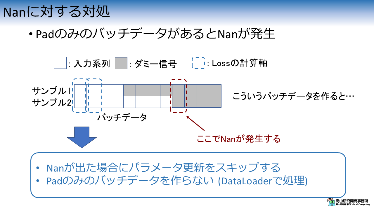
この現象が起きる過程は下記のようになります.
例えば,データセットの最長ラベル系列が分かっていて,その長さに合わせてバッチデータを作成すると,図2に示すようなパッチデータが作成される場合があります.

時系列認識で Cross-entropy loss を計算する場合は,時間軸に沿って1列づつデータを取り出して平均 Loss を計算します.
通常,パディング信号は計算から除外しますので,パディング信号のみデータから平均 Loss を計算しようとすると,Zero 除算によって Nan が発生します.

この問題の対処は単純で,

  • Nan が出た場合に パラメータ更新をスキップする.
  • Pad のみのバッチデータを作らない.

のどちらかの方法で対処ができます.

1番目の方法では,学習ループ時に判定して処理を分岐させればよいです.

2番目の方法では,バッチを作成する際に取り出したサンプルの最大長を用いてパディングを行います.
最低でも 1 サンプルはパディングされないデータが含まれるようになります.
PyTorch では,DataLoader に与えるバッチデータ作成関数で実装できます.

3. ラベル系列長を用いたLossの正規化

時系列認識ではサンプル毎に長さが異なるため,バッチデータを形成して時間軸に沿ってループ処理を行います.
この場合,単純に処理を行うと図3に示すような問題が発生します.

図3: ラベル系列長を用いたLossの正規化
ラベル系列長を用いたLossの正規化

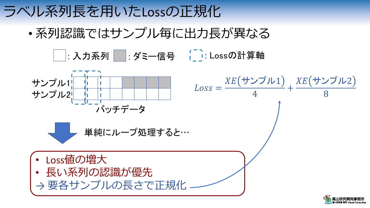
1個目の問題は,Loss 値が系列長に比例して増大する点です.
学習ができなくなるわけではないですが,学習率の調整が必要になるため少し苦労します.

2個目の問題は,長い系列の認識が優先される点です.
長い系列ほど Loss 値が大きくなるため,結果として長い系列の影響が強く出ます.

この問題に対処するためには,各サンプルの長さで Loss を正規化する必要があります.

考え方はシンプルですが,PyTorch には時系列認識向けの Cross-entropy 処理が実装されていないため,自前で処理を組む必要があります.

4. 検証コードによる現象の確認

ここまでに説明した内容を,簡単な検証コードを用いて確認してみます.

4.1 前準備

モジュールのインポート

まず最初に下記のモジュールをインポートします.
(torch だけでできますが,最初に numpy で使って実装してしまったので,そのまま使っています(^^;))

1
2
3
import numpy as np
import torch
from torch import nn

テストデータ作成処理

次に下記のコードでテストデータ作成関数を実装します.

 1
 2
 3
 4
 5
 6
 7
 8
 9
10
11
12
13
14
15
16
17
def create_test_data(samples, vocaburary, max_seqlen, lengths, sos, eos, pad):
    tokens = []
    for length in lengths:
        token = np.random.randint(low=0, high=vocaburary-4, size=length).tolist()
        token = [sos] + token + [eos]
        if len(token) < max_seqlen:
            token += [pad] * (max_seqlen - len(token))
        assert len(token) == max_seqlen
        tokens.append(token)
    tokens = np.array(tokens)

    logits = np.random.rand(samples, max_seqlen, vocaburary)

    # Convert to tensor.
    tokens = torch.from_numpy(tokens)
    logits = torch.from_numpy(logits)
    return logits, tokens
【コード解説】
- 引数
  - samples: サンプル数.
  - vocaburary: ラベルの種類数.
  - max_seqlen: ラベル系列の最大長.
  - lengths: 各ラベル系列の長さ.
  - sos: <sos>のラベル数値.
  - eos: <eos>のラベル数値.
  - pad: <pad>のラベル数値.
- 2-10行目: ラベル系列作成処理.
  ランダムな数値でラベル系列を作成し,先頭と末尾に<sos>と<eos>を加えています.
  `len(token) < max_seqlen` の場合は,<pad> を加えてパディングを行います.
- 12行目: ラベル応答値作成処理.

この処理を実行すると,ラベル系列と予測応答値の系列が作成されます (値はランダムです).

ロス計算処理

次に,下記のコードでロスの計算処理を実装します.

 1
 2
 3
 4
 5
 6
 7
 8
 9
10
11
12
13
def compute_loss(loss_fn, logits, tokens):
    total_loss = 0
    seqlen = tokens.shape[-1]
    for t_index in range(1, seqlen):
        # Skip sos.
        logit = logits[:, t_index-1, :]
        token = tokens[:, t_index]
        loss = loss_fn(logit, token)
        if torch.isnan(loss).any():
            message = f"t_index:{t_index},\n logit:{logit},\n token:{token}"
            raise ValueError(message)
        total_loss += loss
    return total_loss
【コード解説】
- 引数
  - loss_fn: ロス関数.
  - logits: 予測応答値の系列.
  - tokens: ラベル系列.
- 4-12行目: Loss 算出処理.
  - 6-7行目: ラベルと応答値の取り出し.
    ラベルと応答値で,取り出すインデクスがズレている点に注意してください.
  - 8-11行目: Loss の計算.
    Nan が発生している場合は例外を出します.
  - 12行目: 合計の Loss を計算.

上記の処理を実行すると系列全体の Loss が計算されます.
第1節で説明したように,5-6 行目でラベルと応答値を取り出すインデクスをズラしている点に注意してください.

4.2 検証実験

Nanが発生するラベル系列

では,実際にパディング処理の結果 Nan が発生するか確認してみます.
今回は下記の設定でデータを作成します.

1
2
3
4
5
6
7
8
samples = 5
vocaburary = 13
sos = vocaburary - 3
eos = vocaburary - 2
pad = vocaburary - 1
max_seqlen = 10

lengths = np.random.randint(low=1, high=max_seqlen-2, size=samples)
  • サンプル数: 5
  • ラベルの種類数: 13 (キーワードを含む)
  • \(\text{<sos>}\), \(\text{<eos>}\), \(\text{<pad>}\) のラベル数値: 10, 11, 12
  • ラベル系列の最大長: 10

Nan が発生するようにラベル系列長を調整してデータを作成します.

1
2
3
4
5
6
7
lengths[lengths >= max_seqlen-2] = max_seqlen - 3
print(f"lengths of each sample:{lengths}")
# Create tokens.
logits, tokens = create_test_data(samples, vocaburary, max_seqlen, lengths,
                                  sos, eos, pad)
print(f"Shape of logits:{logits.shape}")
print(f"Tokens:{tokens}")
lengths of each sample:[1 4 4 1 7]
Shape of logits:torch.Size([5, 10, 13])
Tokens:tensor([
        [10,  7, 11, 12, 12, 12, 12, 12, 12, 12],
        [10,  7,  2,  6,  3, 11, 12, 12, 12, 12],
        [10,  2,  5,  8,  6, 11, 12, 12, 12, 12],
        [10,  7, 11, 12, 12, 12, 12, 12, 12, 12],
        [10,  0,  7,  3,  1,  8,  6,  7, 11, 12]])

ラベル系列 (Tokens) の出力に注目すると,末尾のラベル数値が全て \(\text{<pad>}=12\) になっています.

このデータを使用して Cross-entropy loss を計算してみます.

1
2
3
4
5
6
7
# Loss using torch's loss naively.
loss_fn = nn.CrossEntropyLoss(reduction="mean", ignore_index=pad)
try:
    total_loss = compute_loss(loss_fn, logits, tokens)
except ValueError as inst:
    print(type(inst))
    print(inst)

上の処理を実行すると,下記のように例外が発生します.

<class 'ValueError'>
t_index:9,
 logit:tensor([[0.7386, 0.8174, 0.4781, 0.3421, 0.3473, 0.1825, 0.6945, 0.9416, 0.7304,
         0.5974, 0.8548, 0.8837, 0.9911],
        [0.3916, 0.8218, 0.8661, 0.0806, 0.1843, 0.8687, 0.0383, 0.5186, 0.5755,
         0.6036, 0.0056, 0.9520, 0.8710],
        [0.2006, 0.0670, 0.2543, 0.7280, 0.1952, 0.3569, 0.8069, 0.5103, 0.6062,
         0.6632, 0.6908, 0.5337, 0.5922],
        [0.4315, 0.1115, 0.7362, 0.1653, 0.4379, 0.2354, 0.2940, 0.7597, 0.1779,
         0.4765, 0.2929, 0.9695, 0.7164],
        [0.1547, 0.9560, 0.9570, 0.2473, 0.9292, 0.9928, 0.7379, 0.5321, 0.2880,
         0.4683, 0.9939, 0.6641, 0.1857]], dtype=torch.float64),
 token:tensor([12, 12, 12, 12, 12])

例外が発生している箇所 (t_index) とラベル配列 (token) を確認すると,ラベル数値が全て \(\text{<pad>}=12\) の箇所であることが分かります.

Lossが系列長に比例する現象

第3節で説明した,Loss がラベル系列長に比例する現象を確認します.

Nan が発生しないようにラベル系列長を調整して,再度データを作成します.

1
2
3
4
5
6
7
lengths[-1] = max_seqlen - 2
print(f"lengths of each sample:{lengths}")
# Create tokens.
logits, tokens = create_test_data(samples, vocaburary, max_seqlen, lengths,
                                  sos, eos, pad)
print(f"Shape of logits:{logits.shape}")
print(f"Tokens:{tokens}")
lengths of each sample:[1 4 4 1 8]
Shape of logits:torch.Size([5, 10, 13])
Tokens:tensor([
        [10,  3, 11, 12, 12, 12, 12, 12, 12, 12],
        [10,  0,  2,  4,  1, 11, 12, 12, 12, 12],
        [10,  7,  2,  2,  7, 11, 12, 12, 12, 12],
        [10,  7, 11, 12, 12, 12, 12, 12, 12, 12],
        [10,  3,  2,  3,  3,  2,  8,  6,  6, 11]])

今回のデータは,最後のラベル系列が末尾まで認識対象ラベルで埋まっているため,Nan は発生しません.

このデータを使用して Cross-entropy loss を計算してみます.

1
2
3
4
5
6
loss_fn = nn.CrossEntropyLoss(reduction="mean", ignore_index=pad)
try:
    total_loss = compute_loss(loss_fn, logits, tokens)
except ValueError as inst:
    print(inst)
print(f"Total loss (Naive):{total_loss}")
Total loss (Naive):23.74435060258172

無事 Loss の計算ができました.
しかし,値をみると \(23.7...\) とかなり大きな値 (孤立手話単語認識では \(2\) から \(3\) 程度でした) で,系列長に比例して値が大きくなっていることが分かります.

系列長を用いたLossの正規化

まず最初に思いつく対策は,下記のように最大系列長で Loss を正規化することだと思います.

1
print(f"Total loss (Normalized by max_seqlen):{total_loss / max_seqlen}")
Total loss (Normalized by max_seqlen):2.374435060258172

値は孤立手話単語認識の場合と同程度になりました.

しかし,最大系列長で正規化した場合は,サンプル間の相対的な Loss 値の比は変わらないため,長い系列が優先される問題は解決していません.

この問題に対処するためには,nn.CrossEntropyLoss クラス内で平均を求めるのを止めて,外部で計算を行う必要があります.
次のコードでは nn.CrossEntropyLoss が生の Loss 値を返すように設定しています.

1
2
3
4
5
6
loss_fn = nn.CrossEntropyLoss(reduction="none", ignore_index=pad)
try:
    total_loss = compute_loss(loss_fn, logits, tokens)
except ValueError as inst:
    print(inst)
print(f"Total loss (Raw):{total_loss}")

nn.CrossEntropyLoss のインスタンス化時に,reduction=none としている点に注意してください.
このように設定すると,各サンプルの Loss 値がそのまま返るようになります.
上記のコードを実行すると,次の結果が得られます.

Total loss (Raw):tensor([
    5.1811,
    12.1516,
    13.7290,
    4.9788,
    24.1034], dtype=torch.float64)

Loss 計算対象のラベル系列長は,\(\text{<eos>}\) を含めるとそれぞれ [2, 5, 5, 2, 9] なので,確かに系列長に比例していることが再度確認できます.

では,Loss を各サンプルの系列長で正規化してみます.

1
2
total_loss /= (lengths + 1)  # Add <eos>.
print(f"Total loss (Normalized by samples lengths):{total_loss}")
Total loss (Normalized by samples lengths):tensor([2.5905, 2.4303, 2.7458, 2.4894, 2.6782], dtype=torch.float64)

無事,各サンプルの Loss 値が同程度になりました.

最後に Loss の平均値を求めれば学習に使える Loss 値が得られます.

1
2
total_loss = total_loss.mean()
print(f"Total loss (Averaged after normalized):{total_loss}")
Total loss (Averaged after normalized):2.58683802922493

4.3 正規化処理のクラス化

正規化処理は少し煩雑なので,学習ループ内に実装するとコードが複雑になってしまいます.
このような場合は,nn.CrossEntropyLoss のようにクラス化しておくと良いでしょう.

 1
 2
 3
 4
 5
 6
 7
 8
 9
10
11
12
13
14
15
16
17
18
19
20
21
22
23
24
25
26
27
28
29
30
31
32
33
34
35
36
37
38
39
40
41
42
43
44
45
46
47
48
49
50
51
52
53
54
55
56
57
58
59
60
61
62
63
64
65
66
67
68
69
70
71
72
73
74
75
76
77
78
79
80
81
82
83
84
85
86
87
88
89
90
91
92
93
94
95
96
97
class LabelSmoothingCrossEntropyLoss(nn.Module):
    """Cross-entropy loss with label smoothing.

    For the detail, please refer
    "Rethinking the Inception Architecture for Computer Vision"
    https://arxiv.org/abs/1512.00567
    """
    def __init__(self, weight=None, ignore_indices=None, reduction="none",
                 label_smoothing=0.0):
        super().__init__()
        self.weight = weight
        if isinstance(ignore_indices, int):
            self.ignore_indices = [ignore_indices]
        else:
            self.ignore_indices = ignore_indices
        assert reduction in ["none",
                             "mean_batch_prior", "mean_temporal_prior",
                             "sum"]
        self.reduction = reduction
        assert label_smoothing >= 0.0
        assert label_smoothing <= 1.0
        self.label_smoothing = label_smoothing

    def _isnotin_ignore(self, target):
        ignore = torch.tensor(self.ignore_indices, dtype=target.dtype,
                              device=target.device)
        isin = (target[..., None] == ignore).any(-1)
        return isin.bitwise_not()

    def _calc_loss(self, logit_t, target_t):
        logit_mask = torch.ones(logit_t.shape[-1],
                                dtype=logit_t.dtype,
                                device=logit_t.device)
        target_mask = torch.ones(target_t.shape,
                                 dtype=logit_t.dtype,
                                 device=logit_t.device)
        if self.ignore_indices is not None:
            logit_mask[self.ignore_indices] = 0
            target_mask = self._isnotin_ignore(target_t).float()
        if self.weight is None:
            weight = torch.ones(logit_t.shape[-1],
                                dtype=logit_t.dtype,
                                device=logit_t.device)
        else:
            weight = self.weight.to(dtype=logit_t.dtype, device=logit_t.device)
        # Calculate CE.
        logprobs = F.log_softmax(logit_t, dim=-1)
        logprobs_m = logprobs * weight * logit_mask
        nll_loss = -logprobs_m.gather(dim=-1, index=target_t.unsqueeze(1))
        nll_loss = nll_loss.squeeze(1)
        smooth_loss = -logprobs_m.sum(dim=-1) / logit_mask.sum()
        smooth_loss *= target_mask
        loss = (1 - self.label_smoothing) * nll_loss + self.label_smoothing * smooth_loss
        return loss

    def forward(self, logit, target):
        """Perform forward computation.

        # Args:
          - logit: `[N, C]` or `[N, C, T]`
          - target: `[N]` or [N, T]
        """
        # Check format.
        if len(logit.shape) == 2:
            logit = logit.unsqueeze(-1)
        if len(target.shape) == 1:
            target = target.unsqueeze(-1)
        assert len(logit.shape) == 3, f"{logit.shape}"
        assert len(target.shape) == 2, f"{target.shape}"
        assert logit.shape[0] == target.shape[0], f"{logit.shape, target.shape}"
        assert logit.shape[-1] == target.shape[-1], f"{logit.shape, target.shape}"

        loss = 0
        for t in range(target.shape[-1]):
            _loss = self._calc_loss(logit[:, :, t], target[:, t])
            # Reduction should be conducted in a loop when reduction is
            # mean_batch_prior.
            if self.reduction == "mean_batch_prior":
                if self.ignore_indices is not None:
                    denom = len([t for t in target[:, t]
                                 if t not in self.ignore_indices])
                else:
                    denom = logit.shape[0]
                _loss /= max(denom, 1)
            loss += _loss

        # Reduction.
        if self.reduction == "sum":
            loss = loss.sum()
        # Temporal Normalization.
        if self.reduction == "mean_batch_prior":
            loss = loss.sum() / target.shape[-1]
        if self.reduction == "mean_temporal_prior":
            target_lengths = self._isnotin_ignore(target).sum(dim=-1)
            loss /= torch.clamp(target_lengths, min=1)
            loss = loss.mean()
        return loss
【コード解説】
- 引数
  - weight: 認識対象ラベルに対する重み.
    使用する場合は認識クラス数の配列で与えます.
  - ignore_indices: Loss の計算対象から除外するインデクスを指定.
  - reduction: Loss 計算の処理方法.
    - none: サンプル毎の Loss 値をそのまま返します.
    - sum: バッチ内の 合計 Loss 値を返します.
    - mean_batch_prior: 各時刻でバッチ内の 平均 Loss 値を求め,足し合わせた後に
      バッチの系列長で正規化します.
      nn.CrossEntropyLoss において `reduction=mean` とした場合と同等です.
    - mean_temporal_prior: サンプル毎に 合計 Loss 値を求めた後に,各サンプルの
      系列長で正規化し,最後にバッチ方向に平均値を求めて返します.
  - label_smoothing: 0 以上の場合,Loss 計算においてラベルスムージングを適用します.
- 10-22行目: 初期化処理.
- 24-28行目: 認識対象クラスのインデクス配列作成処理.
- 30-54行目: 1 系列分の Loss 計算処理.
  - 31-39行目: 認識対象外のクラスを除外するマスク配列を作成.
  - 40-45行目: 重み付け用の配列を作成.
  - 47-53行目: Cross-entropy を計算.
- 64-96行目: 系列全体の Cross-entropy を計算.
  - 64-71行目: フォーマットチェック
  - 73-85行目: Loss 計算処理.
    - 84行目: `reduction = mean_batch_prior` の場合は,ゼロ除算による Nan を
      避けるために 1 以上の値で割るようにしています.
  - 88-96行目: `reduction` の設定に応じて最終的な Loss を計算.

このクラスは内部でループ処理を行うため,系列全体を入力することができます.
ただし,ラベル系列と応答値のインデクス調整は呼び出し側で行う必要がありますので注意してください.

1
2
3
4
5
6
loss_fn = LabelSmoothingCrossEntropyLoss(
    ignore_indices=pad, reduction="mean_temporal_prior")
# `[N, T, C] -> [N, C, T]`
logits = torch.permute(logits, [0, 2, 1])
total_loss = loss_fn(logits[:, :, :-1], tokens[:, 1:])
print(f"Total loss (LabelSmoothingCrossEntropyLoss): {total_loss}")
Total loss (LabelSmoothingCrossEntropyLoss): 2.58683802922493

今回は時系列認識で Loss 計算をする際にハマり易い箇所を紹介しましたが,如何でしたでしょうか?
分かってしまえばどうという程でもないですが,慣れないうちはエラーや性能低下の原因が分からずに悩んでしまうかもしれません (私のことです(^^;)).

時系列認識の実装は複雑な場合が多いので,今後も補足記事などでカバーできたら良いなと思っています.
今回紹介した話が,これから深層学習を勉強してみようとお考えの方に何か参考になれば幸いです.